∮ Riemann Sums

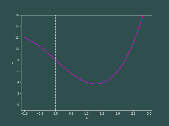
Integration is the act of finding the area under a curve. Let us consider the following function, \begin{equation} f(x) = x^3 - 5x + 8 \end{equation}

Now say I ask you what the area under this curve is from $x=0$ to $x=2$. Surely this is easy enough to solve analytically. $$ A=\int_0^2(x^3-5x+8)dx = \left[\frac{1}{4}x^4 - \frac{5}{2}x^2 + 8x\right]_{x=0}^{x=2}= 10 $$

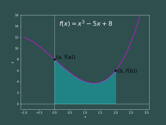
So, the shaded region in the graph above has an area of 10. This is great for a nice function that is so easily solved analytically. However, one often finds themselves dealing with functions that might not be so easily solved with the human mind alone, so how could we compute this area numerically?

An obvious first choice is to do a Riemann sum. Let us break the interval from $x=a$ to $x=b$ up into $N$ rectangles that have height $f(x_i)$ where $x_i$ is the x-coordiate of the $i^{th}$ rectangle, and they have a width of $$ h = \frac{b-a}{N} $$ Then we could approximate the area under the curve to be \begin{equation} A\approx h\sum_{i=0}^{N-1}f(x_i) \end{equation} where $hf(x_i)$ is the area of the $i^{th}$ rectangle -- adding up the areas of all $N$ rectangles yields an approximation of the area under the curve.

In our case, $a=0$ and $b=2$. For simplicity sake, lets take $N=4$ such that $h=0.5$.

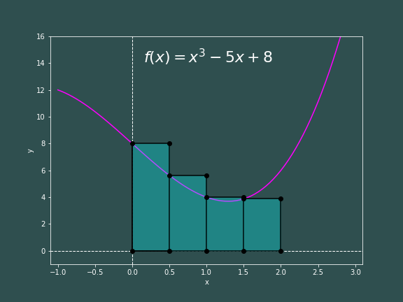
So finding the approximated area under the curve is as simple as applying equation (2) \begin{flalign*} A\approx h\sum_{i=0}^{3} f(x_i) & = h\left(f(x_0) + f(x_1) + f(x_2) + f(x_3) \right)&\\ & = h\left(f(0) + f(0.5) + f(1) + f(1.5) \right) = 10.75 \end{flalign*} Not too bad, only around a 7% error. Obviously, the larger value of $N$ that you choose, the more accurate your approximation will be. It is easy to get your computer to do it for you, here is one way to accomplish this in C++.

        #include <iostream>   // functions for command line interaction
#include <mathETC.h>   // my own math library, you can unclude <cmath>
       
/* define our function to get outputs from inputs
we want the output to be a double, but no need for
long double -- this gives us 8bytes of storage*/
double func(double x)
{
    // int_power(base, exponent) is from my math library 
    double to_return = int_power(x, 3) - 5 * x + 8;
    return to_return;
}

/* define a function that computes Riemann sums.
    First parameter is the function we integrate
    note the first double is the output dataype of
    the function, (&f) is the referene to the function,
    and (double) is telling C++ that f takes a double
    in as a parameter               */                  
    
// a = interval start; b = interval end; N = steps
double riemannSum(double (&f)(double), const float a, const float b, const int N)
{
    // step size
    const double h = (b - a) / N;  

    // compute the integral - note that our termination condition is i<b
    double area = 0;
    for (float i = a; i < b; i += h)
    {
        area += h * func(i);
    }
    
    // return our result
    return area;
}

int main()
{
    // establish parameters
    const float a = 0.0;            // interval start
    const float b = 2.0;            // interval end
    const int N = 4;                // steps

    double area = riemannSum(func, a, b, N);
    std::cout << "Using " << N << " steps, we approximate the area under the curve to be " << area << std::endl;

    return 0;
}

Setting $N=4$, we get the following output from compiling the code above:

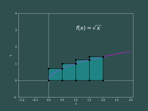
Great! This means we probably have not made an error. Let us investigate the error of Riemann sums a bit more. What we described above is a so-called Left Riemann sum ($A_L$), since the heigh of our rectangles are decided by the value of our function at the left side of the rectangle. Well, one can define a Right Riemann sum ($A_R$) where the height of the rectangle is determined by the value of the function at the right of the rectangles. It can be said that for some increasing function $f(x)$, $$ A_{L} \leq \int_a^b f(x)dx \leq A_{R} $$ where $$ A_L=h\sum_{i=0}^{N-1} f(x_i) \qquad \quad \text{and} \qquad \quad A_R=h\sum_{i=1}^Nf(x_i) $$ This can be "proved" by inspection of the following pictures.

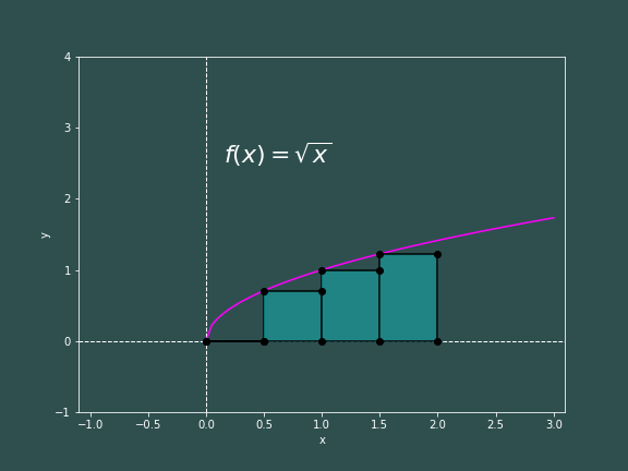
Now if instead $f(x)$ were a decreasing function, we could say $$ A_R \leq \int_a^b f(x)dx \leq A_L $$

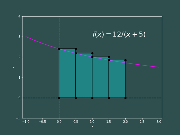
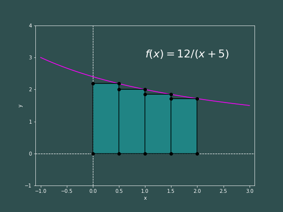
Since one of our Riemann sums is an underestimate, and the other is an overestimate; this means that our error $\epsilon$ can be no more than the difference between the sums. $$ \epsilon \leq \|A_R - A_L\| $$ So, what is the difference between the sums? $$ A_R - A_L = h\left[\sum_{i=0}^{N-1} f(x_i) - \sum_{i=1}^Nf(x_i) \right] $$ \begin{equation*} A_R - A_L = h\left[\left(f(x_0) + f(x_1) + \dotsb + f(x_{N-1}) \right)\\ - \left(f(x_1) + \dotsb + f(x_{N-1}) + f(x_N) \right) \right] \end{equation*} $$ A_R-A_L = h [f(x_0)-f(x_N)] = h[f(a)-f(b)] $$ $$ \|A_R-A_L\| = h \|f(b)-f(a)\| $$ What a clean result! Hence, we have $$ \epsilon \leq h \|f(b)-f(a)\| \qquad \Rightarrow \qquad \epsilon \leq \frac{b-a}{N}\|f(b)-f(a)\| $$ So, if you give me some value of epsilon as an accuracy requirement, I can tell you how many steps we must use: $$ N = \frac{b-a}{\epsilon}\|f(b)-f(a)\| $$ Notice that the number of steps is inversely proportional to the error. So if you want the error to decrease by an order of magnitude, I have to increase the number of steps by an order of magnitude.

Let us now run the code for increasing values of $N$ and see how quickly we converge to 10.

It does indeed seem that our analysis was correct -- to decrease the error by a factor of 10, the number of steps must be increased by a factor of 10.

In the next module we will talk about the trapezoidal rule, which is still conceptually tame, but tends to be much more accuracte than Riemann sums.