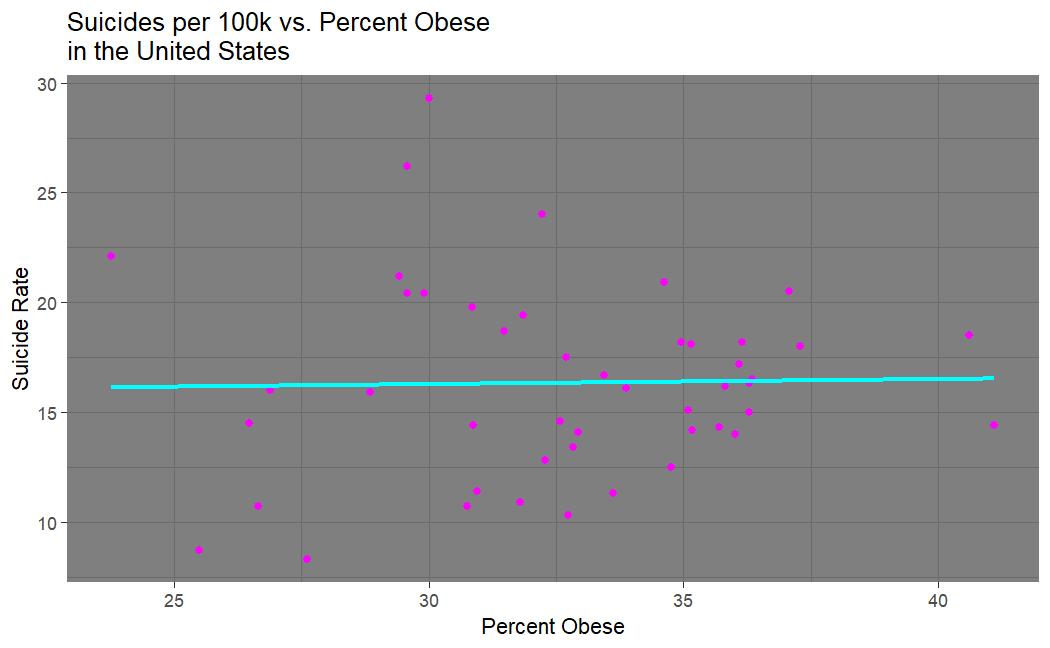
The question I was orginally interested in is whether or not there is a correlation between one's physical health and their mental health. For example, is the obesity rate of a state a decent indicator of that state's suicide mortality rate? I hypothesized that there would be a (ironically) positive correlation between obesity and depression, and between depression and suicide, and therefore between obesity and suicide -- that is, as obesity rates go up, so do rates of depression and suicide.
To answer this I pulled some data sets from the CDC website. The first dataset is about Obesity Rates. This is a very large file that reports the results from survey questions such as "Percent of adults aged 18 years and older who have obesity" from different communities (in 2019) throughout most of the 50 states and many US territories. However, it is missing information about NJ, for example. To get obesity rates for a given state, an average of rates from each district within a state was taken (see code below).
The next dataset I pulled from the CDC webstie was about Suicide Rates (in 2019). This file is was much easier to deal with because it only reports suicide rates (unlike the previous dataset which asks many questions that are tangentially related to obesity). The file reports the suicide rates by city, so again an average of the rates in all cities from a given state was taken to find the suicide rate for that state.
The final dataset pulled from the CDC website holds the results of surveys given in districts throughout the states, asking questions about Depression Rates (in 2017). This might be disingenuous of me to claim, since the question I am using to gauge depression is "Mental health not good for >=14 days among adults aged >=18 Years". These rates were reported by city, so another average has to be taken to find the depression rates by state.
These three data sets were cleaned by picking out the questions of interest, only including the contenintal US (minus NJ since information was missing), and finding the rates of x by state via averaging over rates by district/city; all while being cautious to remove NaN datatypes. The Clean Data Set has a column for stateID, percent of population who are obese, suicides per 100k people, and percent of population who are depressed (or at least reported to have poor mental health for 14 or more of the previous days). See the following block of code to see how this was accomplished.
            import pandas as pd

# function to remove undesired states from data
def remove_states(my_df, state_index, states_list):
   for row, item in my_df.iterrows():
         if item[state_index] not in states_list:
            my_df = my_df.drop(row)
   return my_df

# create a function that averages the values for a given list of entries
def average_entry(my_df, state_index, entry_index):
   check_state = 'AL'
   running_avg = 0
   n = 1
   averages = []
   for row in my_df.itertuples():
         if (row[state_index] in states) and not pd.isna(row[entry_index]):
            if (row[state_index] == check_state) and not (pd.isna(row[entry_index])):
               n += 1
               running_avg += row[entry_index]
            elif (row[state_index] != check_state) and (row[state_index] in states):
               averages.append(round(running_avg/n,2))
               n = 1
               running_avg = row[entry_index]
               check_state = row[state_index]
            else:
               pass
   averages.append(round(running_avg/n,2))
   return averages

# Read CSV file into DataFrame df
df = pd.read_csv('./obesityRates.csv')
df_suicide = pd.read_csv('./suicideRates.csv')
df_depression = pd.read_csv('./depressionRates.csv')

# only take columns of interest
df = df.loc[:,['YearStart','LocationAbbr','Question','Data_Value']]
df_suicide = df_suicide.loc[:, ['YEAR', 'STATE', 'RATE']]
df_depression = df_depression.loc[:, ['StateAbbr', 'Data_Value']] #All 2017

# only consider 2019
df = df[df.YearStart == 2019]
df_suicide = df_suicide[df_suicide.YEAR == 2019]

# get a series of all state accronyms (continental US!)
states = []
check = ['AK', 'DC', 'GU', 'HI', 'PR', 'US', 'NJ']
for i in df.LocationAbbr:
   if i not in check:
         states.append(i)
         check.append(i)
   else:
         pass

# remove undesired states
df = remove_states(df,1,states)
df_suicide = remove_states(df_suicide, 1, states)
df_depression = remove_states(df_depression, 0, states)

# questions
df0 = df[df.Question == 'Percent of adults aged 18 years and older who have obesity']

# alphabetize by state abbreviation
df0 = df0.sort_values('LocationAbbr')
df_suicide = df_suicide.sort_values('STATE')
df_depression = df_depression.sort_values('StateAbbr')

# average the rates of obesity over all age groups
averages_obesity = average_entry(df0,2,4)

# average the rates of depression over all entries for a given state
averages_depression = average_entry(df_depression,1,2)

# put suicide rates in a list to add to desired df, so it doesn't match by index
suicide_rates = []
for r in df_suicide.RATE:
   suicide_rates.append(r)

df_avg = pd.DataFrame([])

df_avg['State'] = states
df_avg['Percent_Obese'] = averages_obesity
df_avg['Suicides_Per_100k'] = suicide_rates
df_avg['Percent_Depressed'] = averages_depression

df_avg.to_csv('cleanDataNew.csv')
Looking at our suicide vs. obesity plot (made in R), we see that my hypothesis was incorrect. There does not seem to be any correlation between suicide and obesity.

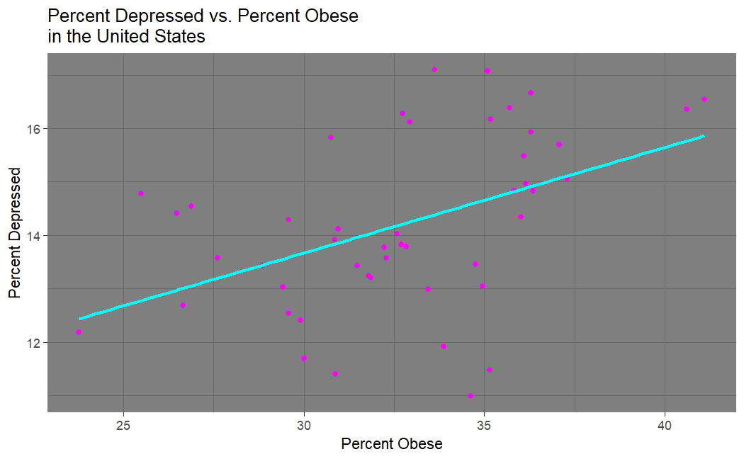
Looking at our depression vs. obesity plot, we see that there does seem to be a strong correlation between being obese and being depressed... this was originally expected, but seems unituitive after seeing that there is no correlation between suicide and obesity. This makes one wonder if there really is a connection between depression and suicide.
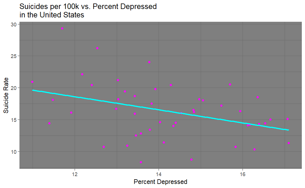
What a fascinating result our suicide vs. depression plot shows! There is a negative correlation between being depressed and committing suicide. So, you are less likely to commit suicide when in a depressive state than you are when you are not in a depressive state; at least based on these data sets. I suspect this is a product of surveying bias -- if I am a depressed person seriously contemplating suicide, how likely am I to participate in one of these surveys about my mental health? This could also very well be due to my decision to equate self-reported "poor mental health" to depression. Truly all we can take from this result is that if you are willing to report that you have poor mental health, you are less likely to commit suicide.
At this point, I decided to plot these items of interest on a map of the United States.
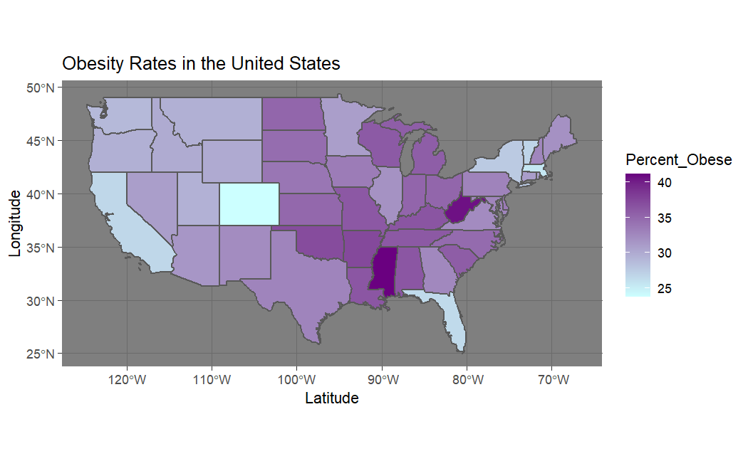
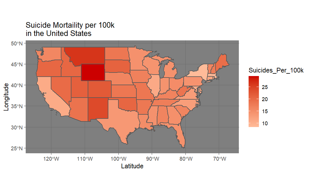
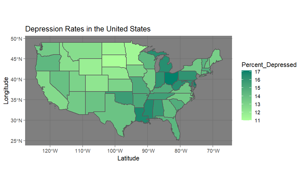
In all cases we appear to have spatial autocorrelation. This led me to write my own program to calculate the Moran's I statistic to get a more rigorous gauge of this spatial autocorrelation.
Moran's I can be calculated by the follwing equation.
\begin{equation}
I=\frac{n}{s_0}\frac{\sum_i\sum_j w_{ij}(Y_i - \bar{Y})(Y_j - \bar{Y})}{\sum_i (Y_i - \bar{Y})^2}
\end{equation}
$$
I\in [-1,1]
$$
Where $n$ is our sample size, $S_0=\sum_i\sum_jw_{ij}$, $Y_i$ is the $i^{\text{th}}$ observed value, and $\bar{Y}$ is the expected value. $w$ is our weight matrix as defined by Gittleman and Kot.
\[
w_{ij}=
\begin{cases}
\frac{1}{d_{ij}} & \qquad d_{ij}\leq c\\
0 & \qquad d_{ij}>c
\end{cases}
\]
I have let $d_{ij}$ be the distance between state $i$ and state $j$, where $c$ is some distance chosen to be the furthest a state can be from another state while having a nonzero weight. Note that I have chosen to not use the typical queen/rook case, even though this is considered to not be best practice. However, I found that my results are quite comparable to the output of running a Moran's I test for the queen case in R.
This is easy enough to implement, but things get a bit more tricky if we want to calculate the p-value for this statistic. To accomplish this, we must find the Z-statistic as follows. $$ Z = \frac{\text{Observed}(I) - \text{Expected}(I)}{\sqrt{\text{V}(I)}} $$ Where V($I$) is the variance, and Expected($I$) = -1/($n-1$). Here is the expression for the variance: $$ \text{V}(I) = \frac{ns_1 - s_2s_3}{(n-1)(n-2)(n-3)(\sum_i\sum_jw_{ij})^2} $$ \begin{multline*} s_1 = (n^2-3n+3)\left(\frac{1}{2}\sum_i\sum_j(w_{ij} + w_{ji})^2\right) \\- n\left[\sum_i\left(\sum_jw_{ij} + \sum_jw{ji}\right)^2\right] +3\left[\sum_i\sum_jw_{ij}\right]^2 \end{multline*} $$ s2 = \frac{n^{-1}\sum_i(Y_i - \bar{Y})^4}{\left(n^{-1}\sum_i(Y_i-\bar{Y})^2\right)^2} $$ \begin{multline*} s_3 = \frac{1}{2}\sum_i\sum_j\left(w_{ij} + w_{ji}\right)^2 - 2n\left[\frac{1}{2}\sum_i\sum_j\left(w_{ij} + w_{ji}\right)^2 \right] + 6\left[\sum_i\sum_jw_{ij} \right]^2 \end{multline*} Which looks horrendous, but is actually quite straightforward to code. Below I provide a "dirty" function for computing the variance that is very inefficient, but it is easy to see how I am computing each term. In the final codeblock for this task I provide a more optomized version of this function (note that both functions still run in $O(n^2)$ time complexity).
# create a function for the variance of moran's I test with maximum readability
def var_morans_I_dirty(column, avg, w):
   n = len(column)

   # first term in s1
   s1_one = 0
   i = 0
   j = 0
   while i < n:
         while j < n:
            s1_one += (w[i][j] + w[j][i])**2
            j += 1
         j = 0
         i += 1
   s1_one *= 0.5*(n**2 - 3*n + 3)

   # second term in s1
   s1_two = 0
   i = 0
   j = 0
   while i < n:
         w_left = 0
         w_right = 0
         while j < n:
            w_left += w[i][j]
            w_right += w[j][i]
            j += 1
         s1_two += (w_left + w_right)**2
         j = 0
         i += 1
   s1_two *= n

   # third term in s1
   s1_three = 0
   i = 0
   j = 0
   while i < n:
         while j < n:
            s1_three += w[i][j]
            j += 1
         j = 0
         i += 1
   s1_three = 3*(s1_three**2)

   # find s1
   s1 = s1_one - s1_two + s1_three

   # s2
   s2_top = 0
   s2_bottom = 0
   for i in column:
         s2_top += (i - avg)**4
         s2_bottom += (i - avg)**2
   s2_top = s2_top/n
   s2_bottom = (s2_bottom/n)**2
   s2 = s2_top/s2_bottom

   # s3
   s3_one = 0
   s3_two = 0
   s3_three = 0
   i = 0
   j = 0
   while i < n:
         while j < n:
            s3_one += (w[i][j] + w[j][i])**2
            s3_two += (w[i][j] + w[j][i])**2
            s3_three += w[i][j] # this will be reused in denominator of V(I)
            j += 1
         j = 0
         i +=1
   s3 = 0.5*s3_one - 2*n*0.5*s3_two + 6*(s3_three**2)

         # finally find the variance
   var_numer = n*s1 - s2*s3
   var_denom = (n-1)*(n-2)*(n-3)*(s3_three**2)
   var = var_numer/var_denom
   return var
Now I will provide the finalized code that outputs the Moran's I test for obesity rates, suicide rates, and depression rates in the United States. Here is the .shp file used to find the distances between each state usaMap.
import geopandas as gpd
import pandas as pd
import numpy as np
import scipy.stats

# create a function for the variance of moran's I
def var_morans_I(column, avg, w):
   n = len(column)
   wij = 0
   wij_wji_sq = 0
   s1_two = 0
   i = 0
   j = 0
   while i < n:
         w_left = 0
         w_right = 0
         while j < n:
            wij += w[i][j]
            wij_wji_sq += (w[i][j] + w[j][i])**2
            w_left += w[i][j]
            w_right += w[j][i]
            j += 1
         s1_two += (w_left + w_right)**2
         j = 0
         i += 1
   s1_one = wij_wji_sq*0.5*(n**2 - 3*n + 3)
   s1_two *= n
   s1_three = 3*wij**2
   s3_one = 0.5*wij_wji_sq
   s3_two = n*wij_wji_sq
   s3_three = 6*wij**2

   s1 = s1_one - s1_two + s1_three
   s3 = s3_one - s3_two + s3_three

   # s2
   s2_top = 0
   s2_bottom = 0
   for i in column:
         s2_top += (i - avg)**4
         s2_bottom += (i - avg)**2
   s2_top = s2_top/n
   s2_bottom = (s2_bottom/n)**2
   s2 = s2_top/s2_bottom

   # finally find the variance
   var_numer = n*s1 - s2*s3
   var_denom = (n-1)*(n-2)*(n-3)*(wij**2)
   var = var_numer/var_denom
   return var


# create a function for morans i test
def morans_I(column, avg, w):
   n = len(column)
   s_0 = 0
   i = 0
   j = 0
   numerator = 0
   denominator = 0
   while i < n:
         denominator += (column[i]-avg)**2
         while j < n:
            s_0 += w[i][j]
            numerator += w[i][j]*(column[i]-avg)*(column[j]-avg)
            j += 1
         j = 0
         i += 1
   coeff = n/s_0
   moran_I = coeff*numerator/denominator

   # now find the p-value
   expected_value = -1/(1-n)
   #var = var_morans_I_dirty(column, avg, w)
   var = var_morans_I(column, avg, w)
   std = np.sqrt(var)
   z_score = (moran_I - expected_value)/std
   p_value = scipy.stats.norm.sf(abs(z_score))
   return moran_I, p_value

map_df = gpd.read_file('./usaMap/States_shapefile.shp')

# get a series of all state accronyms (continental US!)
states = []
check = ['AK', 'DC', 'GU', 'HI', 'PR', 'US', 'NJ']
for i in check:
   map_df = map_df[map_df.State_Code != i]

# add centroids
map_df['centroid'] = map_df.centroid

# alphabetize by state_code
map_df = map_df.sort_values(by=['State_Code'])

# weight matrix
w_ij = []
i = 0
j = 0
c = 8
n = len(map_df['State_Name'])
while i < n:
   row_to_add = []
   while j < n:
         if i == j:
            row_to_add.append(0)
            j += 1
         else:
            dist = (map_df['centroid'].iloc[j].distance(map_df['centroid'].iloc[i]))
            if dist <= c:
               to_add = 1/dist
            else:
               to_add = 0
            row_to_add.append(to_add)
            j += 1
   # normalize row before adding to weight matrix
   row_to_add_norm = [float(i)/sum(row_to_add) for i in row_to_add]
   w_ij.append(row_to_add_norm)
   j = 0
   i += 1


# import clean data
data = pd.read_csv('cleanData.csv')
data = data.sort_values(by='State')

# calculate averages
i = 0
obese_avg = 0
suicide_avg = 0
depressed_avg = 0
while i < n:
   obese_avg += data['Percent_Obese'].iloc[i]
   suicide_avg += data['Suicides_Per_100k'].iloc[i]
   depressed_avg += data['Percent_Depressed'].iloc[i]
   i += 1
obese_avg /= n
suicide_avg /= n
depressed_avg /= n

# test morans I function
obesity_morans_I, obesity_p_value = morans_I(data['Percent_Obese'], obese_avg, w_ij)
suicide_morans_I, suicide_p_value = morans_I(data['Suicides_Per_100k'], suicide_avg, w_ij)
depressed_morans_I, depressed_p_value = morans_I(data['Percent_Depressed'], depressed_avg, w_ij)

print("Obesity Moran's I: ", obesity_morans_I, "    p-value: ", obesity_p_value)
print("Suicide Moran's I: ", suicide_morans_I, "    p-value: ", suicide_p_value)
print("Depression Moran's I: ", depressed_morans_I, "    p-value: ", depressed_p_value)
Here is our output (I have rounded):
The null hypothesis for the Moran's I test is that our data is randomly dispersed. Since our p-values are statistically significant, we reject this null hypothesis. This provides a strong indication that we do indeed have positive spatial autocorrelation for obesity rates, suicide rates, and depression rates in the United States.
Gittleman, John L., and Mark Kot. "Adaptation: statistics and a null model for estimating phylogenetic effects." Systematic Zoology 39.3 (1990): 227-241.
Plant, Richard E. Spatial data analysis in ecology and agriculture using R. cRc Press, 2018.