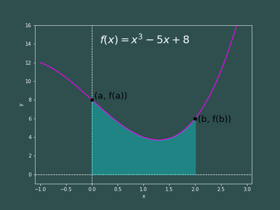
Consider the same function we wanted to integrate from the module on Riemann Sums, $$ f(x) = x^3 - 5x +8 $$ And again, we would like to find the area under this curve from $x=0$ to $x=2$.

Analytically, we find that $$ A = \int_{x=0}^{x=2}\left(x^3-5x+8\right)dx = \left[\frac{1}{4}x^4-\frac{5}{2}x^2 + 8x\right]_{x=0}^{x=2} =10 $$ We have already tried numerically solving this integral using Riemann sums, so let us now try using the trapezoidal rule. We can get a closer approximation to the area under the curve by summing up the areas of $N$ trapezoids, compared to the lousy rectangles of Riemann.
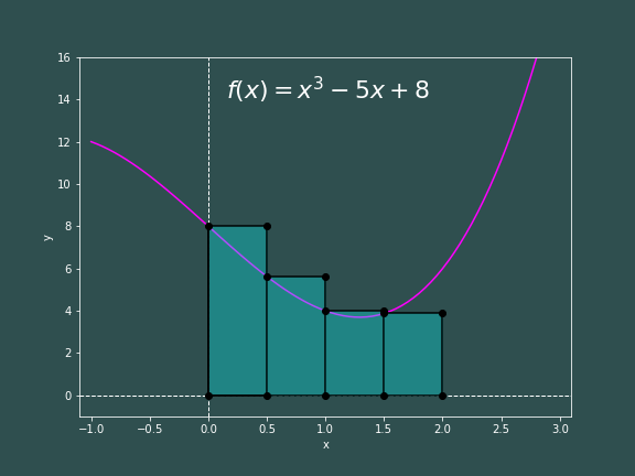
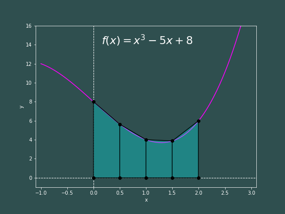
Like last time, we will break the interval from $x=a$ to $x=b$ up into $N$ chunks, such that each slice has a width of
$$
h = \frac{b-a}{N}
$$
The right hand side of the $k^{\text{th}}$ slice falls at $x=a+kh$ and its left hand side falls at $x=a+kh-h = a + (k-1)h$
The area of a trapezoid can be derivied easily enough. Consider the trapezoid $k=0$, it has width $h=(b-a)/N$, and lets say it has a base $b_0=f(x_0)$ and another base $b_1=f(x_1)$. Clearly, we can split this up into a rectangle and a right triangle. Now our task is to find the areas of the rectangle and the triangle, and add them together to get the area of the entire trapezoid.
$$
A_{trap} = hb_0 + \frac{1}{2}h(b_1 - b_0) = hb_0 + \frac{1}{2}hb_1 - \frac{1}{2}hb_0 = \frac{1}{2}h(b_0 + b_1)
$$
In this case,
$$
A_1 = \frac{1}{2}h(f(x_0)+f(x_1)) = \frac{1}{2}h(f(a) + f(a + h))
$$
Which is easily generalized to the $k^{\text{th}}$ trapezoid
$$
A_k = \frac{1}{2}h(f(a + (k-1)h)+f(a + kh))
$$
Then to get a numerical approximation of the area under the curve, we need to sum up the area of all $N$ trapezoids.
\begin{flalign*}
A = \sum_{k=1}^NA_k &= \frac{1}{2} h \sum_{k=1}^N \left[f(a+(k-1)h) + f(a+kh)\right] \\
&= \frac{1}{2} h \left[f(a) + f(a+h) + f(a+h) + f(a+2h) + f(a+2h) + \ldots + f(b) \right] \\
&= h\left[\frac{1}{2}f(a) + \frac{1}{2}f(b) + f(a + h) + f(a+2h) + \ldots + f(a+(N-1)h)\right] \\
&= h\left[\frac{1}{2}f(a) + \frac{1}{2}f(b) + \sum_{k=1}^{N-1}f(a+kh) \right]
\end{flalign*}
This is the so-called extended trapezoidal rule, hereby denoted as merely the trapezoidal rule.
\begin{equation}
\int_{x=a}^{x=b}f(x)dx \approx h\left[\frac{1}{2}f(a) + \frac{1}{2}f(b) + \sum_{k=1}^{N-1}f(a+kh) \right]
\end{equation}
It is interesting to note that the area approximation is dependent on the value of our function at every sample point we generate in our plight for discretization -- but it gives the end points a weight of 0.5, and the internal points a weight of 1.
Let's say that $x_k = a + kh$ and consider a slice of the integral
$$
\int_a^b f(x)dx
$$
that falls between $x_{k-1}$ and $x_k$,
$$
\int_{x_{k-1}}^{x_k}f(x)dx
$$
Why not try taking a Taylor expansion of $f(x)$ about $x_{k-1}$?
\begin{flalign*}
f(x) = f(x_{k-1}) &+ (x-x_{k-1})f'(x_{k-1}) + \frac{(x-x_{k-1})^2}{2!}f''(x_{k-1})\\
&+ \frac{(x-x_{k-1})^3}{3!}f'''(x_{k-1}) + \ldots
\end{flalign*}
$$
\Rightarrow f(x) = \sum_{j=0}^{\infty}\frac{(x-x_{k-1})^j}{j!}\frac{d^jf(x)}{dx^j}\bigg|_{x=x_{k-1}}
$$
We want to find the area under the curve from $x_k$ to $x_{k-1}$, so we integrate.
\begin{flalign*}
\int_{x_{k-1}}^{x_n} f(x)dx = f(x_{k-1})\int_{x_{k-1}}^{x_k} dx &+ f'(x_{k-1})\int_{x_{k-1}}^{x_k} (x-x_{k-1})dx\\
&+ \frac{f''(x_{k-1})}{2}\int_{x_{k-1}}^{x_k}(x-x_{k-1})^{2} dx\\
&+ \frac{f'''(x_{k-1})}{6}\int_{x_{k-1}}^{x_k}(x-x_{k-1})^{3}dx + \ldots
\end{flalign*}
$$
\Rightarrow \int_{x_{k-1}}^{x_n} f(x)dx = \int_{x_{k-1}}^{x_n}\sum_{j=0}^{\infty}\frac{(x-x_{k-1})^j}{j!}\frac{d^jf(x)}{dx^j}\bigg|_{x=x_{k-1}}dx
$$
Now we can use a u-substitution where
$$
u = x-x_{k} \qquad \qquad du = dx
$$
and our bounds of integration become $u(x=x_{k-1})=0$ and $u(x=x_k)=x_k - x_{k-1} = h$. So the integral now becomes,
$$
\int_{x_{k-1}}^{x_n} f(x)dx = \int_{0}^{h}\sum_{j=0}^{\infty}\frac{u^j}{j!}\frac{d^jf(x)}{dx^j}\bigg|_{x=x_{k-1}}du
$$
\begin{flalign*}
\Rightarrow\int_{x_{k-1}}^{x_n} f(x)dx = f(x_{k-1})\int_{0}^{h} du &+ f'(x_{k-1})\int_{0}^{h} udu\\
&+ \frac{f''(x_{k-1})}{2}\int_{0}^{h}u^{2} du\\
&+ \frac{f'''(x_{k-1})}{6}\int_{0}^{h}u^{3}du + \ldots
\end{flalign*}
\begin{flalign*}
\Rightarrow \int_{x_{k-1}}^{x_n} f(x)dx = h f(x_{k-1}) + \frac{h^2}{2}f'(x_{k-1}) + \frac{h^3}{6}f''(x_{k-1}) +O(h^4)
\end{flalign*}
This is an approximation of the area of the curve for one slice of width $h=x_k - x_{k-1}$ using a Talor expansion about $x_{k-1}$; so we will call this
\begin{equation}
A_{x_{k-1}} = h f(x_{k-1}) + \frac{h^2}{2}f'(x_{k-1}) + \frac{h^3}{6}f''(x_{k-1}) +O(h^4)
\end{equation}
Now we will take the Taylor expansion of out function about $x_n$
\begin{flalign*}
f(x) = f(x_k) + f'(x_k)(x-x_k) &+ \frac{f''(x_k)}{2}(x-x_k)^2\\
&+\frac{f'''(x_k)}{6}(x-x_k)^3 + \ldots
\end{flalign*}
$$
\Rightarrow f(x) = \sum_{j=0}^{\infty}\frac{(x-x_k)^j}{j!}\frac{d^jf(x)}{dx^j}\bigg|_{x=x_k}
$$
Again, we integrate from $x_{k-1}$ to $x_k$.
\begin{flalign*}
\int_{x_{k-1}}^{x_k}f(x)dx = f(x_k)\int_{x_{k-1}}^{x_k}dx &+ f'(x_k)\int_{x_{k-1}}^{x_k}(x-x_k)dx\\
&+ \frac{f''(x_k)}{2}\int_{x_{k-1}}^{x_k}(x-x_k)^2dx\\
&+ \frac{f'''(x_k)}{6}\int_{x_{k-1}}^{x_k}(x-x_k)^3dx + \ldots
\end{flalign*}
$$
\Rightarrow \int_{x_{k-1}}^{x_k}f(x) dx= \int_{x_{k-1}}^{x_k}\sum_{j=0}^{\infty}\frac{(x-x_k)^j}{j!}\frac{d^jf(x)}{dx^j}\bigg|_{x=x_k}dx
$$
And we use a similar u-sibstitution as before, however our bounds of integration are different this time around.
$$
u = x-x_k \qquad \qquad du = dx
$$
With bounds of integration:
$$
u(x=x_{k-1})=x_{k-1}-x_k = -h \qquad \qquad u(x=x_k) = 0
$$
The integral becomes
$$
\int_{x_{k-1}}^{x_k}f(x) dx= \int_{-h}^{0}\sum_{j=0}^{\infty}\frac{u^j}{j!}\frac{d^jf(x)}{dx^j}\bigg|_{x=x_k}du
$$
\begin{flalign*}
\Rightarrow\int_{x_{k-1}}^{x_k}f(x) dx = f(x_k)\int_{-h}^{0}du + f'(x_k)\int_{-h}^{0}udu &+ \frac{f''(x_k)}{2}\int_{-h}^{0}u^{2}du \\
&+ \frac{f'''(x_k)}{6}\int_{-h}^{0}u^3du + \ldots
\end{flalign*}
$$
\Rightarrow \int_{x_{k-1}}^{x_k}f(x) dx= hf(x_k) - \frac{h^2}{2}f'(x_k) + \frac{h^3}{6}f''(x_k)-O(h^4)
$$
This is an approximation of the area of the curve for one slice of width $h=x_k - x_{k-1}$ using a Talor expansion about $x_k$; so we will call this
\begin{equation}
A_{x_k} = h f(x_k) - \frac{h^2}{2}f'(x_k) + \frac{h^3}{6}f''(x_k) - O(h^4)
\end{equation}
Now we average (2) and (3) together to find that
\begin{flalign*}
\bar{A} = \frac{A_{x_k} + A_{x_{k-1}}}{2} = \frac{h}{2}\left[f(x_{k-1}) + f(x_k)\right] &+ \frac{h^2}{4}\left[f'(x_{k-1}) - f'(x_k)\right] \\
&+ \frac{h^3}{12}\left[f''(x_{k-1}) + f''(x_k)\right] + O(h^4)
\end{flalign*}
This is an approximation of the area of a single region of width $h$ under the curve. To find the entire area under the curve within our bounds of interest, we need to sum over all $N$ regions:
\begin{multline*}
\int_a^b f(x)dx = \sum_{k=1}^{N}\int_{x_{k-1}}^{x_k}f(x)dx =\frac{h}{2}\sum_{k=1}^{N} \left[f(x_{k-1}) + f(x_k)\right] +\frac{h^2}{4}\left[f'(a) - f'(b)\right] \\
+ \frac{h^3}{12}\sum_{k=1}^{N}\left[f''(x_{k-1}) + f''(x_k)\right] + O(h^4)
\end{multline*}
The first term on the right hand side is the trapezoidal rule! Which means that when we approximate the area under a curve using the trapezoidal rule, we have an error of
\begin{equation}
\epsilon = \frac{h^2}{4}\left[f'(a) - f'(b)\right] + \frac{h^3}{12}\sum_{k=1}^{N}\left[f''(x_{k-1}) + f''(x_k)\right] + O(h^4)
\end{equation}
Note that the second term on the right hand side is just the trapezoidal rule applied to the integral of the function $f''(x)$ from $x=a$ to $x=b$ (times a constant). That is,
$$
\int_a^bf''(x)dx = \frac{h}{2}\sum_{k=1}^{N}\left[f''(x_{k-1})+f''(x_k)\right] + O(h^2)
$$
Let us try multiplying this by $h^2/6$
$$
\frac{h^2}{6}\int_a^bf''(x)dx = \frac{h^3}{12}\sum_{k=1}^N\left[f''(x_{k-1}) + f''(x_k)\right] + O(h^4)
$$
$$
\Rightarrow \frac{h^3}{12}\sum_{k=1}^N\left[f''(x_{k-1})+f''(x_k)\right] = \frac{h^2}{6}\int_a^bf''(x)dx + O(h^4)
$$
But the integral of $f''(x)dx$ is $f'(x)$, so this becomes
$$
\frac{h^3}{12}\sum_{k=1}^N\left[f''(x_{k-1})+f''(x_k)\right] = \frac{h^2}{6}\left[f'(b)-f'(a)\right] + O(h^4)
$$
Combining this result with equation (4) gives us the following expression for the error.
\begin{flalign*}
\epsilon &= \frac{h^2}{4}\left[f'(a)-f'(b)\right] + \frac{h^2}{6}\left[f'(b) - f'(a)\right] + O(h^4) \\
&= \frac{6h^2}{24}\left[f'(a)-f'(b)\right]- \frac{4h^2}{24}\left[f'(a) - f'(b)\right] + {O(h^4)}
\end{flalign*}
\begin{equation}
\Rightarrow \epsilon = \frac{h^2}{12}\left[f'(a) - f'(b)\right]
\end{equation}
Our long waited result, a second order approximation for our error when we use the trapezoidal rule. This tells us that the trapezoidal rule is a first order integration scheme, accurate to $O(h)$ with an error on the order of $O(h^2)$.
        #include <iostream>      // functions for command line interaction
#include "mathETC.h"     // my own math library, you can include <cmath>

// define a function for our function ;)
double func(double x)
{
    double to_return = int_power(x, 3) - 5 * x + 8;
    return to_return;
}

/* define a function that approximates the integral
    using Trapezoidal rule */
double trap_rule(double(&f)(double), const float a, const float b, const int N)
{
    // step size
    const double h = (b - a) / N;

    // compute integral
    double area = 0.5 * (f(a) + f(b));
    for (double i = 1; i < N; i += 1)
    {
        area += f(a + i * h);
    }

    // return our approximation
    return h*area;
}

int main()
{
    // establish parameters
    const float a = 0.0;            // interval start
    const float b = 2.0;            // interval end
    const int N = 4;                // steps

    double area = trap_rule(func, a, b, N);

    std::cout.precision(12);
    std::cout << "Using " << N << " steps, we approximate the area under the curve to be " << area << std::endl;
}
Here is our output for increasing the number of steps $N$:
We see that our calculations are seeming to converge to 10 as we increase $N$.
    import matplotlib.pyplot as plt

# create a solutions class
class Integrator(object):
    # method for our integral of choice
    def func(self, x):
        return x**3 - 5*x + 8

    # method for the integration
    def trap_rule(self, a,b,N):
        h = (b-a)/N
        area = 0.5*(func(a) + func(b))
        for i in range(1,N):
            area += func(a + i*h)
        return h*area

# initialize parameters
a = 0.0
b = 2.0
N_i = 100
N_f = 1000
trial0 = Integrator()

# lists to fill for plot
areas = []
Ns = []

# iterate over many different values of N
for N in range(N_i, N_f + 1):
    new_area = trial0.trap_rule(a,b,N)
    areas.append(new_area)
    Ns.append(N)

# plot the area approximation vs the number of steps
with plt.rc_context({'axes.edgecolor':'white', 'xtick.color':'white', \
                        'ytick.color':'white', 'figure.facecolor':'darkslategrey',\
                        'axes.facecolor':'darkslategrey','axes.labelcolor':'white',\
                        'axes.titlecolor':'white'}):
    plt.figure(figsize=(10,6))
    plt.xlabel("Number of Steps")
    plt.ylabel("Error in Area")

    # use list comprehension to plot the error in the area vs. N
    plt.plot(Ns, [abs(x-10) for x in areas], color='m')
    plt.savefig("./trap_error.png")
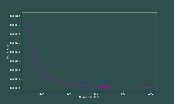
Clearly, our error is approaching zero as $N$ gets larger.