I will be using my datasets talked about in my module on the Moran's I Statistic.
We want to generate a line of best fit between some dependent variable $y$ and some independent (explanatory) variable $x$ for some set of data such that we minimize the sum of the squared residuals. That is, if our line estiates a value $\hat{y}_i$ for some $x_i$; but the observed value is $y_i$, our task is to minimize
\begin{equation}
\sum_{i=1}^n(y_i - \hat{y}_i)^2 = \sum_{i=1}^n\epsilon_i^2
\end{equation}
A given observed value may be written as
\begin{equation*}
y_i = \beta_0 + \beta_1x_i + \epsilon_i
\end{equation*}
where $\epsilon_i$ is some error term (our residual for the $i^{\text{th}}$ observation).
\begin{equation}
\Rightarrow \epsilon_i = y_i - \beta_0 -\beta_1x_i
\end{equation}
The estimators of our ordinary least squares (OLS) parameters $\hat{\beta}_0$ and $\hat{\beta}_1$ must minimize
\begin{equation}
S(\beta_0, \beta_1) = \sum_{i=1}^n(y_i - \beta_0 - \beta_1x_i)^2
\end{equation}
In other words, the following two equations must hold.
\begin{equation}
\frac{\partial S}{\partial \beta_0}\biggr\vert_{\hat{\beta}_0, \hat{\beta}_1} = -2\sum_{i=1}^n (y_i - \hat{\beta}_0 - \hat{\beta}_1x_i) = 0
\end{equation}
\begin{equation}
\frac{\partial S}{\partial \beta_1}\biggr\vert_{\hat{\beta}_0, \hat{\beta}_1} = -2\sum_{i=1}^n (y_i - \hat{\beta}_0 - \hat{\beta}_1x_i)x_i = 0
\end{equation}
Where we have taken the derivatives via the chain rule and set the results equal to zero to find the minimums. From here, we can do some cute algebra to find expressions for $\hat{\beta}_0$ and $\hat{\beta}_1$. Let us first turn our attention to equation (4).
\begin{equation*}
-2\sum_{i=1}^n (y_i - \hat{\beta}_0 - \hat{\beta}_1x_i) = 0
\end{equation*}
\begin{equation*}
\Rightarrow \sum_{i=1}^n (y_i - \hat{\beta}_0 - \hat{\beta}_1x_i) = 0
\end{equation*}
\begin{equation*}
\Rightarrow \sum_{i=1}^n y_i - \sum_{i=1}^n\hat{\beta}_0 - \sum_{i=1}^n\hat{\beta}_1x_i = 0
\end{equation*}
\begin{equation*}
\Rightarrow \sum_{i=1}^n y_i - \sum_{i=1}^n\hat{\beta}_1x_i = n\hat{\beta}_0
\end{equation*}
\begin{equation*}
\Rightarrow \hat{\beta}_0 = \frac{\sum_{i=1}^ny_i - \hat{\beta}_1\sum_{i=1}^nx_i}{n}
\end{equation*}
\begin{equation}
\Rightarrow \hat{\beta}_0 = \bar{y} - \hat{\beta}_1\bar{x}
\end{equation}
What a nice result! The estimator of our y-intercept is the average value of our observed independent variable minus the average of our observed explanatory variable times our estimator of the slope. However, we now need an expression for $\hat{\beta}_1$; so we now will look at equation (5).
\begin{equation*}
-2\sum_{i=1}^n (y_i - \hat{\beta}_0 - \hat{\beta}_1x_i)x_i = 0
\end{equation*}
Using equation (6), this becomes
\begin{equation*}
\Rightarrow \sum_{i=1}^n (y_i - (\bar{y} - \hat{\beta}_1\bar{x}) - \hat{\beta}_1x_i)x_i = 0
\end{equation*}
\begin{equation*}
\Rightarrow \sum_{i=1}^n \left[(y_i - \bar{y}) - \hat{\beta}_1(x_i-\bar{x})\right]x_i = 0
\end{equation*}
\begin{equation*}
\Rightarrow\left[\sum_{i=1}^n(y_i - \bar{y}) - \hat{\beta}_1\sum_{i=1}^n(x_i - \bar{x})\right]\sum_{i=1}^nx_i=0
\end{equation*}
\begin{equation*}
\Rightarrow\left[\sum_{i=1}^n(y_i - \bar{y}) - \hat{\beta}_1\sum_{i=1}^n(x_i - \bar{x})\right]n\bar{x}=0
\end{equation*}
Since $n$ and $\bar{x}$ are constants, we can simplify this
\begin{equation*}
\Rightarrow \sum_{i=1}^n(y_i - \bar{y}) - \hat{\beta}_1\sum_{i=1}^n(x_i - \bar{x})=0
\end{equation*}
\begin{equation}
\Rightarrow \hat{\beta}_1=\frac{\sum_{i=1}^n(y_i-\bar{y})}{\sum_{i=1}^n(x_i-\bar{x})} = \frac{\sum_{i=1}^n(y_i-\bar{y})(x_i-\bar{x})}{\sum_{i=1}^n(x_i-\bar{x})^2}= \frac{S_{xy}}{S_{xx}}
\end{equation}
Where $S_{xy}$ is the covariance between $x$ and $y$; and $S_{xx}$ is the variance of $x$. Again, what a surprisingly nice result! So we can use these estimators to come up with a line of best fit.
$$\hat{\beta}_0 = \hat{y} - \hat{\beta}_1\bar{x}$$
$$\hat{\beta}_1= \frac{\sum_{i=1}^n(y_i-\bar{y})(x_i-\bar{x})}{\sum_{i=1}^n(x_i-\bar{x})^2}= \frac{S_{xy}}{S_{xx}}$$
$$\hat{y} = \hat{\beta}_0 + \hat{\beta}_1\bar{x}=\bar{y}-\hat{\beta}_1\bar{x}+\hat{\beta}_1x$$
\begin{equation}
\Rightarrow \hat{y} = \bar{y} + \frac{S_{xy}}{S_{xx}}(x-\bar{x})
\end{equation}
Now we will derive the goodnes-of-fit, or $R^2$, test. First we must define a few terms. First,
$$
t_i = y_i - \bar{y}
$$
which acts as a measure of how much an observation deviates from the mean. Squaring this term and summing it up over all observations gives us the total sum of squares:
$$
\sum_{i=1}^nt_i^2 = \sum_{i=1}^n(y_i - \bar{y})^2
$$
Secondly,
$$
\Rightarrow \sum_{i=1}^n\eta_i^2 = \sum_{i=1}^n(\hat{y}_i - \bar{y})^2
$$
which is the portion of the total sum of squares that is explained by our regression model.
Finally,
$$
\sum_{i=1}^n\hat{\epsilon}_i^2 = \sum_{i=1}^n (y_i - \hat{y}_i)^2
$$
is our residual sum of squares -- the bit of the data that is not explained by our regression model.
We note that equation (4) can be written as
\begin{equation}
\sum_{i=1}^n\hat{\epsilon}_i = 0
\end{equation}
and equation (5) can be written as
\begin{equation}
\sum_{i=1}^n\hat{\epsilon}_ix_i = 0
\end{equation}
Now we would like to prove the following:
$$
\sum_{i=1}^n\hat{y}_i\hat{\epsilon}_i = 0
$$
Proof: Start with our estimated line of best fit.
$$
\hat{y}_i = \hat{\beta}_0 + \hat{\beta}_1x_i
$$
Multiply both sides of this equation by $\hat{\epsilon}_i$.
$$
\hat{y}_i\hat{\epsilon}_i = \hat{\beta}_0\hat{\epsilon}_i + \hat{\beta}_1x_i\hat{\epsilon}_i
$$
Sum over all $n$ observations.
$$
\sum_{i=1}^n\hat{y}_i\hat{\epsilon}_i = \hat{\beta}_0\sum_{i=1}^n\hat{\epsilon}_i + \hat{\beta}_1\sum_{i=1}^nx_i\hat{\epsilon}_i
$$
Making use of equations (9) and (10) we find our desired result.
\begin{equation}
\sum_{i=1}^n\hat{y}_i\hat{\epsilon}_i = 0
\end{equation}
$\qquad\qquad\qquad\qquad\qquad\qquad$QED
Now we would like to prove that $$ \sum_{i=1}^nt_i^2 = \sum_{i=1}^n\eta_i^2 + \sum_{i=1}^n\hat{\epsilon}_i^2 $$ Proof: \begin{flalign*} \sum_{i=1}^nt_i^2 &= \sum_{i=1}^n(y_i-\bar{i})^2 = \sum_{i=1}^n\left[(\hat{y}_i-\hat{\epsilon}_i) -\bar{y} \right]^2 = \sum_{i=1}^n\left[\hat{\epsilon}_i + (\hat{y}_i-\bar{y})\right]^2 &\\ &= \sum_{i=1}^n \left[\hat{\epsilon}_i^2 + 2\hat{\epsilon}_i(\hat{y}_i-\bar{y}) + (\hat{y}_i - \bar{y})^2 \right] &\\ &= \sum_{i=1}^n\hat{\epsilon}_i^2 + 2\sum_{i=1}^n(\hat{\epsilon}_i\hat{y}_i-\hat{\epsilon}_i\bar{y}) + \sum_{i=1}^n(\hat{y}_i-\bar{y})^2 &\\ &= \sum_{i=1}^n\hat{\epsilon}_i^2 + 2\sum_{i=1}^n\hat{\epsilon}_i\hat{y}_i -2\bar{y}\sum_{i=1}^n\hat{\epsilon}_i + \sum_{i=1}^n\eta_i^2 \end{flalign*} Using equations (9) and (11), we find that the middle two terms cancel and we are left with our desired result. \begin{equation} \sum_{i=1}^nt_i^2 = \sum_{i=1}^n\eta_i^2 + \sum_{i=1}^n\hat{\epsilon}_i^2 \end{equation}
$\qquad\qquad\qquad\qquad\qquad\qquad$QED
To reiterate, $\sum_{i=1}^nt_i^2$ is a gauge of how much variation is found in our response variable; and $\sum_{i=1}^n\eta_i^2$ is a gauge of how much of that variation is explained by our regression model. So, we define the $R^2$ test as
\begin{equation}
R^2 = \frac{\sum_{i=1}^n\eta_i^2}{\sum_{i=1}^nt_i^2} = \frac{\sum_{i=1}^n(\hat{y}_i-\bar{y})^2}{\sum_{i=1}^n(y_i - \bar{y})^2}
\end{equation}
\end{equation}
Making use of equation (12), this can be rewritten in the form that is more typically seen.
\begin{equation}
R^2 = 1 - \frac{\sum_{i=1}^n\hat{\epsilon}_i^2}{\sum_{i=1}^n\eta_i^2} = 1-\frac{\sum_{i=1}^n(y_i - \hat{y}_i)^2}{\sum_{i=1}^n(y_i - \bar{y})^2}
\end{equation}
        import pandas as pd
import matplotlib.pyplot as plt
import numpy as np

# create a function that takes in a column of data and outputs its average
def average_output(column_of_data):
    n = len(column_of_data)
    avg = 0
    i = 0
    while i < n:
        avg += column_of_data.iloc[i]
        i += 1
    avg /= n
    return avg

# create a function that takes in a column of data and outputs the variance
def variance_output(column_of_data):
    n = len(column_of_data)
    xbar = average_output(column_of_data)
    s_xx = 0
    i = 0
    while i < n:
        s_xx += (column_of_data.iloc[i] - xbar)**2
        i += 1
    return s_xx

# create a functino that takes in two columns of data, and outputs their covariance
def covariance_output(x, y):
    n = len(x)
    xbar = average_output(x)
    ybar = average_output(y)
    s_xy = 0
    i = 0
    while i < n:
        s_xy += (y.iloc[i] - ybar)*(x.iloc[i] - xbar)
        i += 1
    return s_xy

# create a function that runs OLS and outputs parameters B_0 and B_1
# returns beta0, beta1, and r^2
def ols_one(x_col, y_col):
    # find beta1 and beta0
    xbar = average_output(x_col)
    ybar = average_output(y_col)
    s_xy = covariance_output(x_col, y_col)
    s_xx = variance_output(x_col)
    beta1 = s_xy/s_xx
    beta0 = ybar - beta1*xbar

    # get yhat points at observations
    estimate_points = []
    i = 0
    for x in x_col:
        yhat = beta0 + beta1*x
        estimate_points.append(yhat)
        i += 1

    r_sq = r_squared(y_col, estimate_points)

    return round(beta0, 4), round(beta1, 4), round(r_sq, 4)

# create a function for finding r^2 value
def r_squared(data, estimate):
    sst = 0           # total sum of squares
    sse = 0           # estimated sum of squares
    n = len(data)
    ybar = average_output(data)
    i = 0
    while i < n:
        sse += (ybar - estimate[i])**2
        sst += (data[i] - ybar)**2
        i += 1

    r_sq = sse/sst
    return r_sq

# import clean data
data = pd.read_csv('cleanDataNew.csv')
data = data.sort_values(by='State')

# run ordinary least squares to find parameters of line of best fit
beta0, beta1, r_sq1 = ols_one(data['Percent_Obese'], data['Percent_Depressed'])
print('beta0 =', beta0, '\nbeta1 =', beta1, '\nr_sq =', r_sq1)
This code produces the following output.
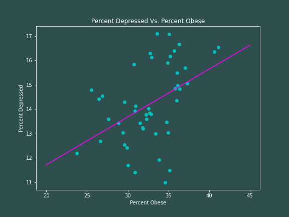
So our ordinary least squares model for depression rates as a function of obesity rates is as follows: $$ \hat{Y} = 7.7914 + 0.1962X $$ with $R^2 = 0.2034$. So based on this model we would expect a state with no obese inhabitants to have 7.8% of its population be depressed, with the depression rate increasing by about 0.2% for every 1% increase in obesity rates. However, our goodness-of-fit test tells us that this is really not a great representation of the data -- there is a lot of variation from our linear model. Here is some code to produce a plot.
    x_min = 20
x_max = 45
domain_hat = np.linspace(x_min, x_max, 500)
yhat = []
for x in domain_hat:
    yhat.append(beta0 + beta1*x)

with plt.rc_context({'axes.edgecolor':'white', 'xtick.color':'white', \
                    'ytick.color':'white', 'figure.facecolor':'darkslategrey',\
                    'axes.facecolor':'darkslategrey','axes.labelcolor':'white',\
                    'axes.titlecolor':'white'}):
    plt.figure(figsize=(8,6))
    plt.plot(data['Percent_Obese'], data['Percent_Depressed'], 'co')
    plt.plot(domain_hat, yhat, color='magenta')
    plt.title("Percent Depressed Vs. Percent Obese")
    plt.xlabel('Percent Obese')
    plt.ylabel('Percent Depressed')
    plt.savefig('../images/obeseVsDepressed_python.png')

Visually, there certainly does appear to be a positive correlation between being depressed and being obese, which is supported by our linear model.
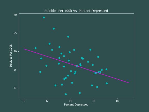
I will now run the above code to model suicide rates as a function of depression -- if you have seen my module on the Moran's I Statistic, you might remember that we get an unexpected result. Using the ordinary least squares method, we find
$$
\hat{Y} = 30.975 - 1.0307X
$$
$$
R^2 = 0.1461
$$

Based on this data and our ordinary least squares model, we would expect a state with no depressed inhabitants to have around 31 suicides per 100k people; and that suicide rate would actually decrease as the percentage of depressed inhabitants increases -- a result that defies intuition. In fact, if we extrapolate beyond a reasonable amount, we would expect that a state with around 31% of its inhabitants having depression would on average have no suicides comitted at all.